Noisy Data? Python Has a Filter for That
A practical intro to Kalman filters
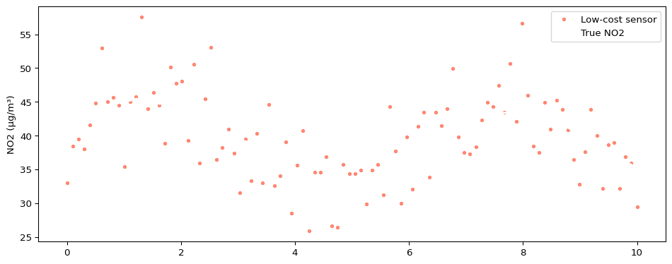
Example: Noisy NO2 Signal
Using the Class
kf = KalmanFilter1D(
    x0=40.0, P0=10.0,
    A=1, H=1,
    Q=0.3, R=25.0
)

estimates = kf.filter(meas)

fig, ax = plt.subplots(figsize=(6, 4))
ax.plot(t, meas,      '.', color="tomato",    label="Sensor",   alpha=0.6)
ax.plot(t, true,      '-', color="white",     label="True NO2", linewidth=2)
ax.plot(t, estimates, '-', color="limegreen", label="Filtered", linewidth=2.5)
ax.set_ylabel("NO2 (μg/m³)")
ax.legend()
plt.tight_layout()
plt.show()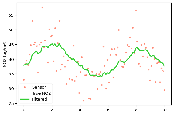
Filter → Smooth
kf2 = KalmanFilter1D(
    x0=40.0, P0=10.0,
    A=1, H=1, Q=0.3, R=25.0
)
kf2.filter(meas)
smoothed = kf2.smooth()

fig, ax = plt.subplots(figsize=(6, 4))
ax.plot(t, meas,           '.', color="tomato",    label="Sensor",   alpha=0.5)
ax.plot(t, true,           '-', color="white",     label="True NO2", linewidth=2)
ax.plot(t, kf2.estimates,  '-', color="limegreen", label="Filtered", linewidth=2, alpha=0.7)
ax.plot(t, smoothed,       '-', color="gold",      label="Smoothed", linewidth=2.5)
ax.set_ylabel("NO2 (μg/m³)")
ax.legend()
plt.tight_layout()
plt.show()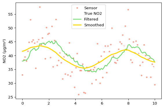
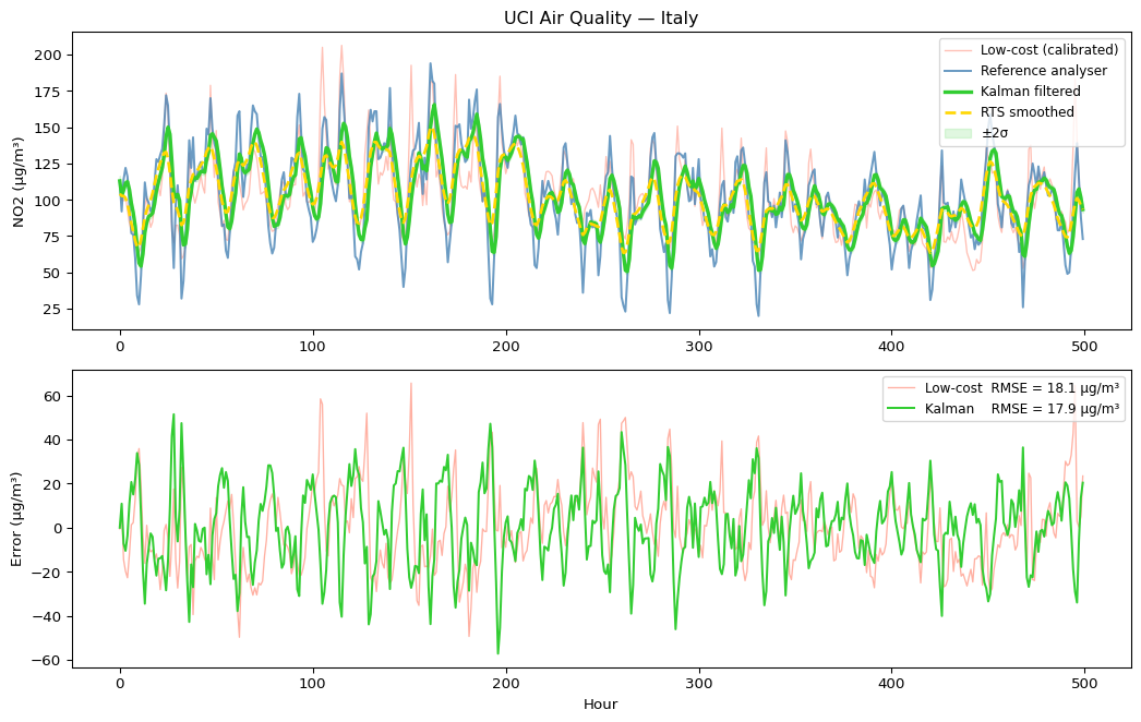
Result: Real Fusion